Technical Data Analysis


Serial Correlation Analysis
In this blog, we show you how to convert OpenDataDSL timeseries into matrices and then perform a serial correlation to show how intra-timeseries correlations can help predict future price movements.
What is Technical Data Analysis?
Technical Data analysis refers to the process of systematically examining and interpreting data using various analytical and statistical techniques to derive insights and draw conclusions. Some common techniques used in data analysis include regression analysis, hypothesis testing, machine learning, data visualization, and data mining. Data analysis can involve several steps, including data collection, cleaning, transformation, modeling, and visualization. The goal is to extract meaningful information from raw data, identify patterns and trends, and use these insights to support the business.
Hourly Electricity Price Data
As an example we use Iberian Electricity data published by OMIE. Specifically we use electricity prices for Spain for the year 2022 on an hourly granularity.
Timeseries visualisation
Visualizing the timeseries of the hourly prices using the ODSL WebPortal
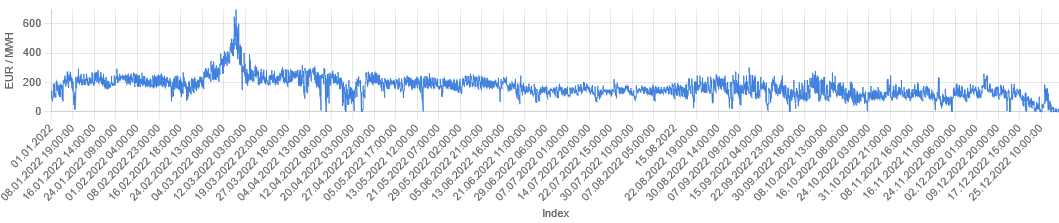
This visualization of time series data is a common way to analyse trends, seasonality, and other patterns that occur over time.
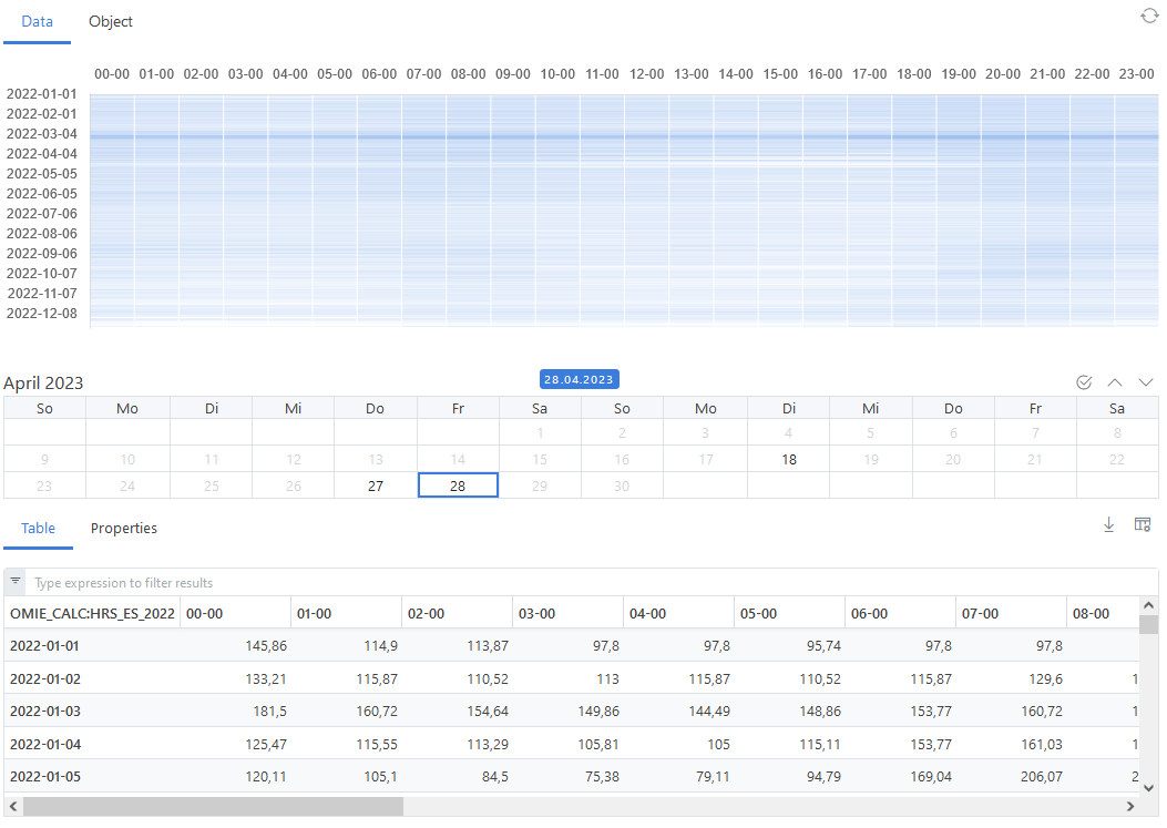
Matrix visualisation
Another way to get insights to the data is to convert this time series into a matrix, where columns represent the hours of the day 1-24 and rows represent the days of the year 1-365. This transformed view supports the task to analyse the same data input but per hour of the day over time. ODSL supports it with a function toMatrix()
// Input time series are the electricity prices for Spain from OMIE for 2022
input = ${data:"#OMIE.EL.ES.DA:PRICE_TS"}
d1 = parse("2022-01-01T00:00:00", "yyyy-MM-dd'T'HH:mm:ss", "Europe/Madrid")
d2 = parse("2022-12-31T23:00:00", "yyyy-MM-dd'T'HH:mm:ss", "Europe/Madrid")
input = input.range(d1, d2)

// transform the time series into a matrix
mx = input.toMatrix(DailyCalendar())
You can visualize the data view in ODSL Web-Portal:
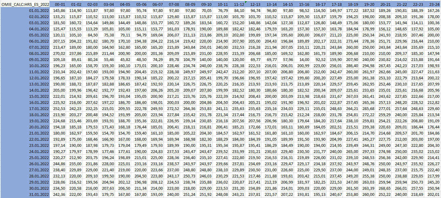
Excel Add-in
You can use our ODSL Excel-Addin to easily view matrix data (here a graphs snipped for the days 1-31 of year 2022):
Correlation
Referring to my latest blog Data - Facts and Figures, we know that correlation analysis helps to identify dependencies in the data set. ODSL supports different input options calculating the Bravais-Pearson correlation coefficients. In the blog Data - Facts and Figures two time series are used.
In this blog, we use a matrix as an input, where the correlation of each of the columns is calculated with all the columns of the matrix. The result is again a matrix. Moreover, the function supports a shift parameter to perform a serial correlation.
Serial correlation
Investopedia describes serial correlation as:
Serial correlation occurs in a time series when a variable and a lagged version of itself (for instance a variable at times T and at T-1) are observed to be correlated with one another over periods of time. Repeating patterns often show serial correlation when the level of a variable affects its future level. In finance, this correlation is used by technical analysts to determine how well the past price of a security predicts the future price.
// set the precision to 4 for rounding
set precision 4
// calculating the correlation using a matrix mx as an input (from above)
// and a shift parameter of 1 or 7:
obj.HRS_ES_2022_d_d1 = correlation(mx, 1)
obj.HRS_ES_2022_d_d7 = correlation(mx, 7)
A use case for this is the correlation matrix from above of a day d against the previous day d-1 when the shift parameter is 1. Obviously you can use any shift parameter - for instance with a shift parameter of 7 you calculate the correlation from today d against previous weeks prices which is d-7.
Heatmap formatting
The matrix output colored as a heatmap using the formatting:
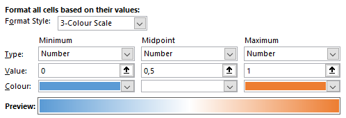
where no correlation is blue, correlation of 50% is colored in white and perfect correlation is colored in orange.
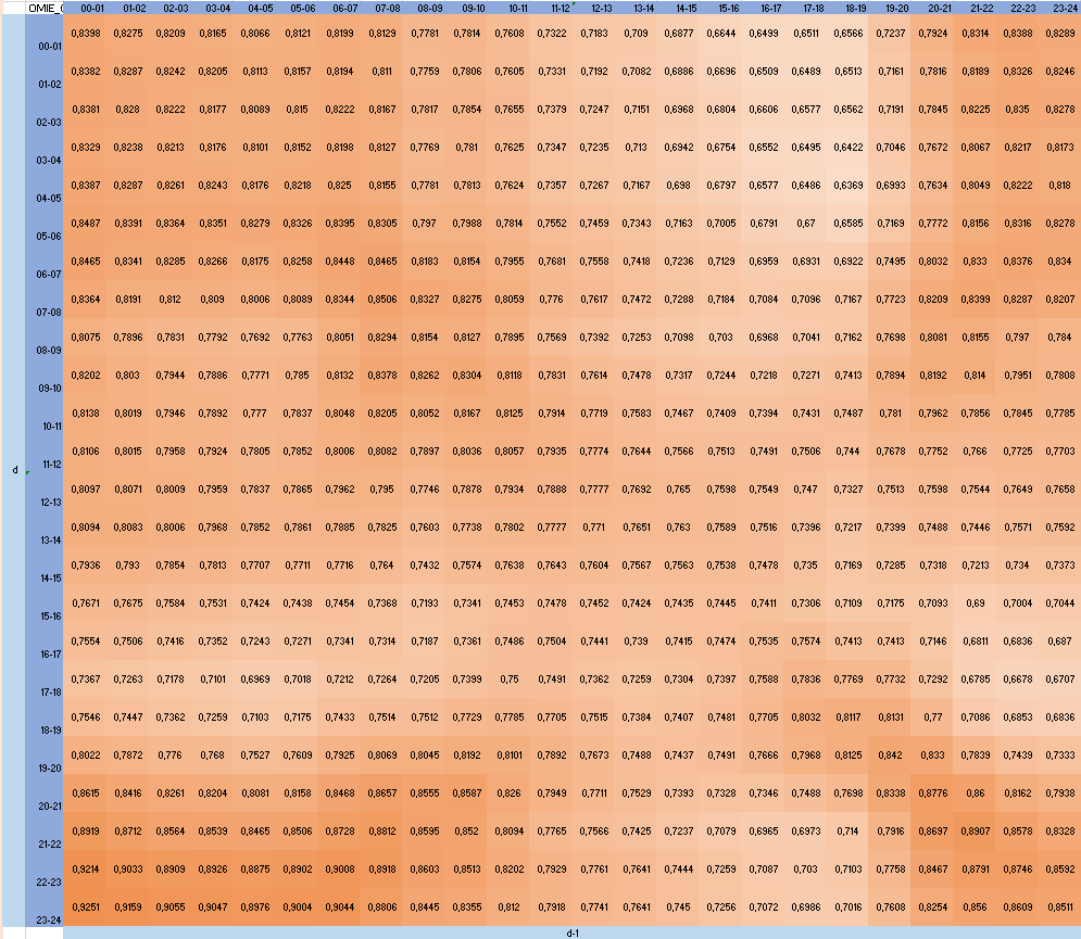
The correlation matrix from day d against d-1:
The correlation between day d and day d-1 of the 24 hours granularity over 364 days range (due to a shift of 1 day) is quite high with correlation coefficients between 63,69% and 92,51%.
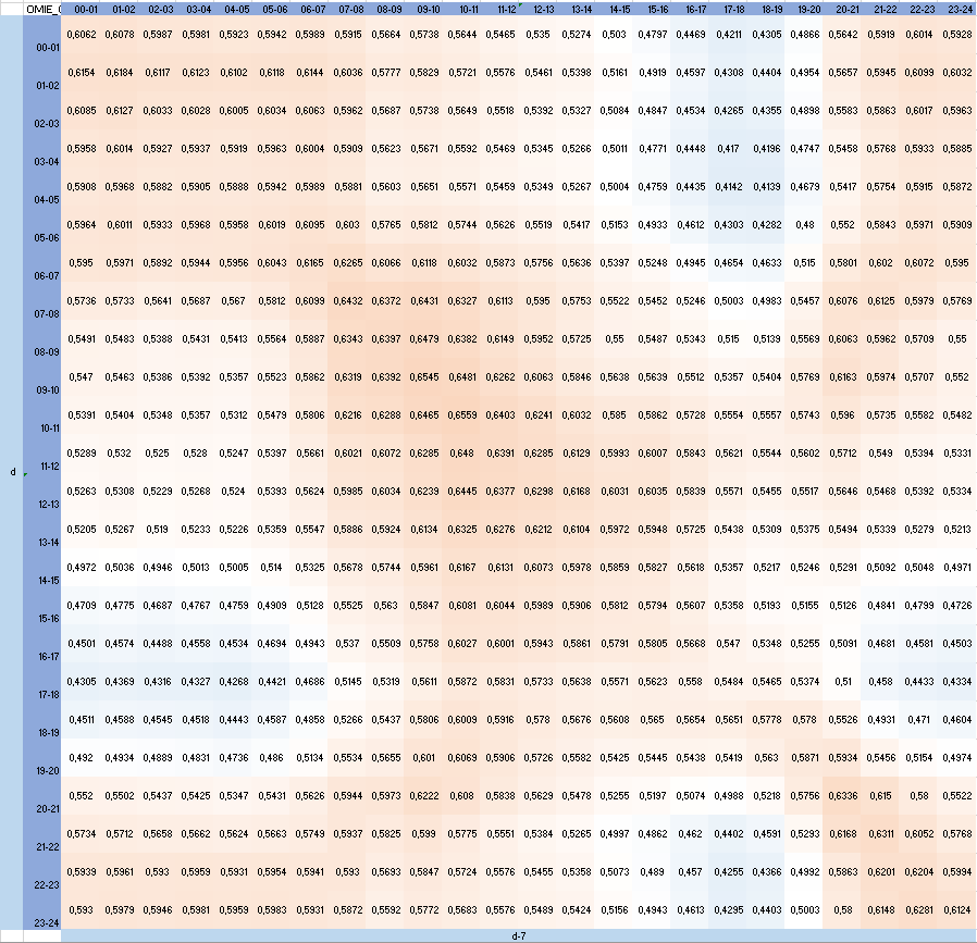
The correlation matrix from day d against d-7:
The correlation between day d and day d-7 of the 24 hours granularity over 358 days range (due to a shift of 7 days) is moderate with correlation coefficients between 41,39% and 65,59%.
Conclusion
Correlation analysis helps to identify dependencies in the data set and serves to setup solid price forecasts, where it is essential to know how the price dependencies is behaving historically with specific investigations for short and long contracts. One use case for it is shaping forward curves.
Next steps
Do you want to see this in action and see how you can benefit from OpenDataDSL?
Fill out the form below, we will contact you to arrange a personally tailored demo.
How about a demo?
Our team is here to find the right solution for you, contact us to see this in action.
Fill out your details below and somebody will be in contact with you very shortly.
More information or free trial?
Tell us about your project, and we can let you know how we can help.
Contact us at info@opendatadsl.com